Detecting quadratic phase coupling from time series data by rhosa
Source:vignettes/quadratic_phase_coupling.Rmd
quadratic_phase_coupling.RmdAbstract
In this vignette we show how to detect quadratic phase coupling (QPC)
of one-dimensional or multi-dimensional real-valued time series by
bicoherence or cross_bicoherence of rhosa,
respectively. The first section gives an example applying
bicoherence to the data from a simple model exhibiting QPC
at each frequency pair. In the second section we describe a generative
model of three channels with another kind of QPC revealed by
cross_bicoherence. The third section summarizes when and
why bicoherence or cross_bicoherence fails to
recognize a certain type of QPC.
A toy model of QPC
We begin with importing rhosa:
Our first mathematical model, adapted from [1], is a superposition of six cosine curves of unit amplitude with different frequencies, named \(x_1\):
\[x_1(t) = \sum_{i=1}^{6} \cos(\lambda_i t + \varphi_i)\]
where, for each \(i = 1,2,...,6\), \(\lambda_i\) is given and fixed, namely
\[ \lambda_1 = 0.55; \lambda_2 = 0.75; \lambda_3 = \lambda_1 + \lambda_2; \] \[ \lambda_4 = 0.6; \lambda_5 = 0.8; \lambda_6 = \lambda_4 + \lambda_5. \]
On the other hand, we choose \(\varphi_i\) (\(i = 1, ..., 5\)) independently from the uniform variable of range \([0, 2\pi)\), and define
\[ \varphi_6 = \varphi_4 + \varphi_5. \]
Note that the trigonometric identities implies
\[\cos(\lambda_6 t + \varphi_6) = \cos((\lambda_4 + \lambda_5) t + (\varphi_4 + \varphi_5)) = \cos(\lambda_4 t + \varphi_4) \cos(\lambda_5 t + \varphi_5) - \sin(\lambda_4 t + \varphi_4) \sin(\lambda_5 t + \varphi_5),\]
so \(\cos(\lambda_6 t + \varphi_6)\) is positively correlated with the product of \(\cos(\lambda_4 t + \varphi_4)\) and \(\cos(\lambda_5 t + \varphi_5)\). But \(\cos(\lambda_3 t + \varphi_3)\) is not correlated with the product of \(\cos(\lambda_1 t + \varphi_1)\) and \(\cos(\lambda_2 t + \varphi_2)\) in general as the phase \(\varphi_3\) is randomly assigned.
Once \(\varphi_i\)s are chosen,
\(x_1(t)\) is a periodic function of
\(t\). So it turns out that \(x_1\) is a (strictly) stationary stochastic
process. The wave length of any frequency component of \(x_1\) is shorter than \(4\pi\). Now consider sampling a realization
of \(x_1\) repeatedly during a fixed
length of time, say 256. The sampling rate is 1. That is, the interval
of consecutive samples is 1. The following R code effectively simulates
\(x_1\) as x1.
triple_lambda <- function(a, b) c(a, b, a + b)
lambda <- c(triple_lambda(0.55, 0.75), triple_lambda(0.6, 0.8))
x1 <- function(k) {
    set.seed(k)
    init_phi <- runif(5, min = 0, max = 2*pi)
    phi <- c(init_phi, init_phi[4] + init_phi[5])
    function(t) do.call(sum, Map(function(l, p) cos(l * t + p), lambda, phi))
}
observe <- function(f) {
    sapply(seq_len(256), f)
}
N1 <- 100
m1 <- do.call(cbind, Map(observe, Map(x1, seq_len(N1))))
Each column of matrix m1 in the last line represents a
realization of x1. That is, we have taken 100 realizations
of \(x_1\) as m1. Let’s
plot them:
ith_sample <- function(i) {
    data.frame(i = i, t = seq_len(256), v = m1[,i])
}
r1 <- do.call(rbind, Map(ith_sample, seq_len(100)))

library(ggplot2)

ggplot(r1) +
    geom_line(aes(t, v)) +
    facet_wrap(vars(i)) +
    theme(axis.title.y = element_blank(),
          axis.text.y = element_blank(),
          strip.background = element_blank(),
          strip.text.x = element_blank())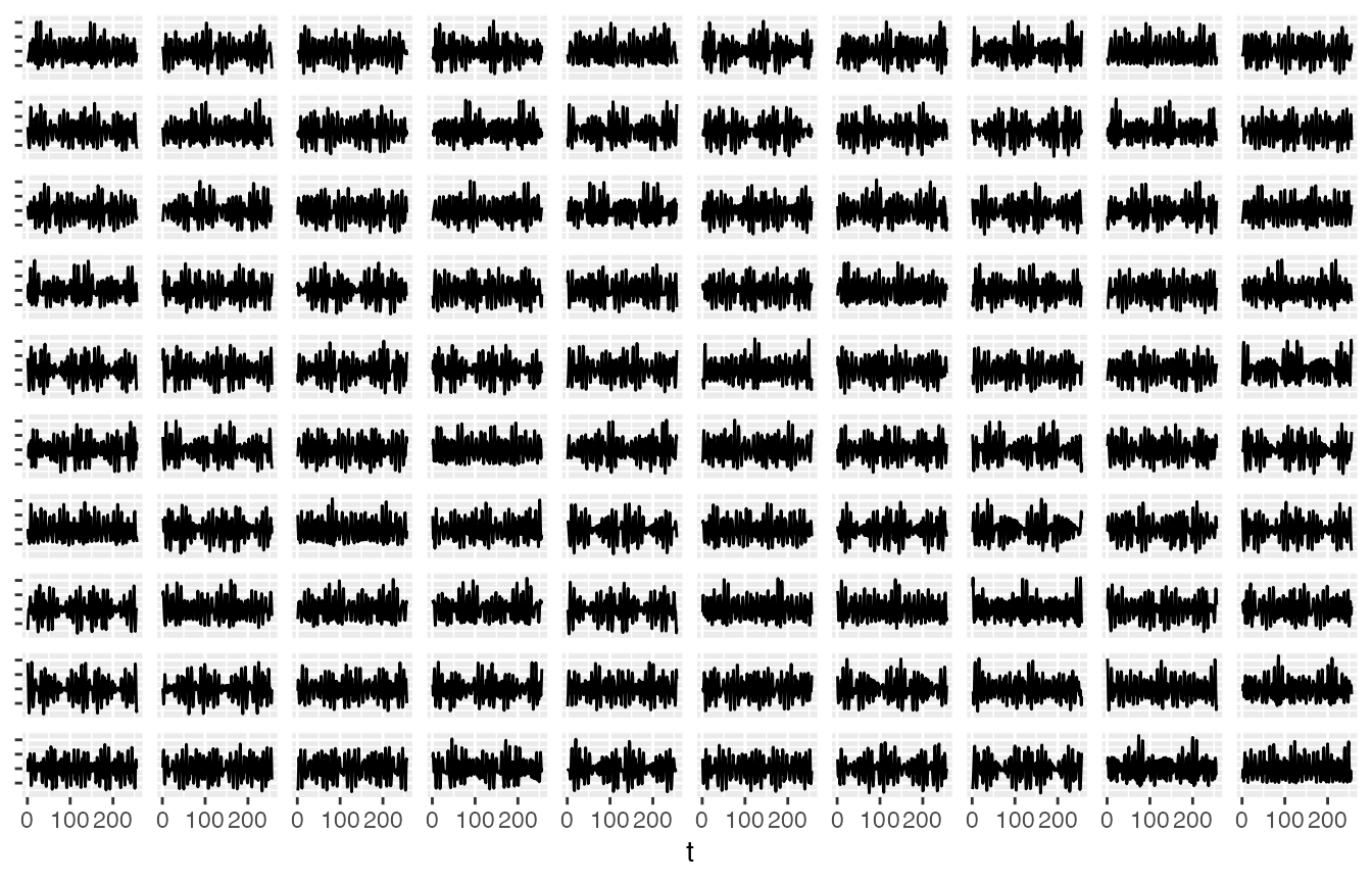
100 realizations of x1.
A realization of \(x_1\) looks like:

The 256 time points in the first realization of x1.
Its spectrum estimation shows peaks at six frequencies as expected:
spectrum(m1)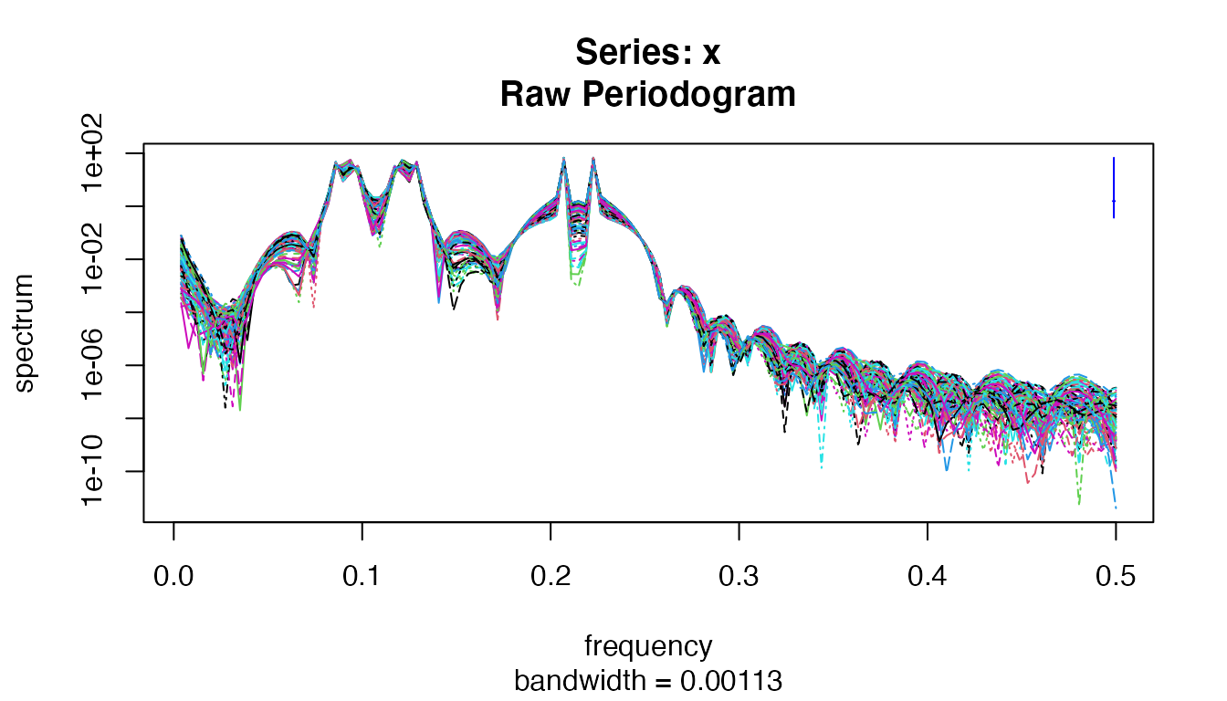
The spectrum estimation of x1.
Now we approximate \(x_1\)’s
bicoherence by bicoherence:
bc1 <- bicoherence(m1)… and define an R function to plot the heat map of the estimated bicoherence:
heatmap_bicoherence <- function(bc) {
    ggplot(bc) +
        geom_raster(aes(f1, f2, fill = value)) +
        coord_fixed() +
        scale_alpha(guide = "none")
}

heatmap_bicoherence(bc1)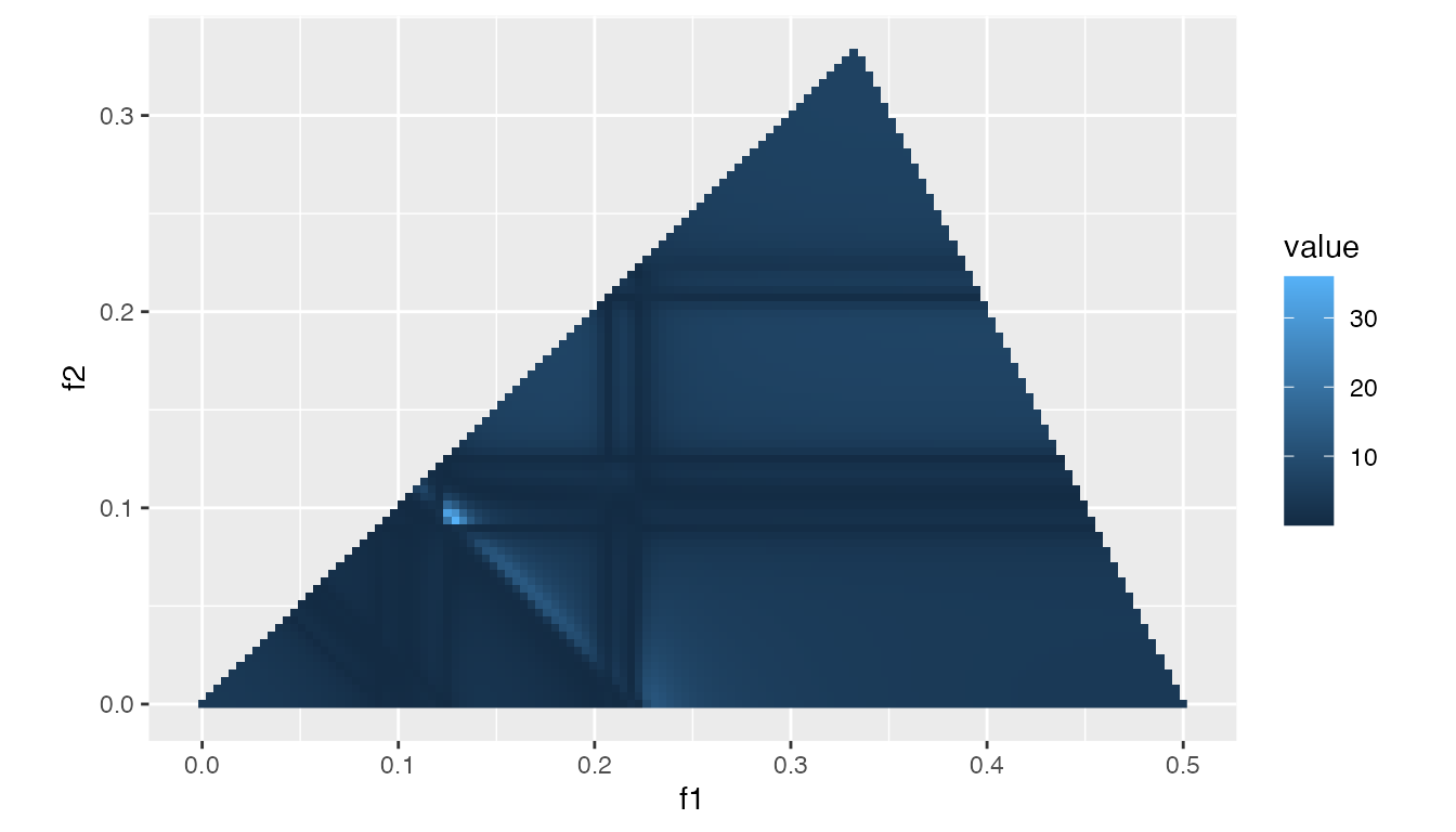
x1’s estimated bicoherence.
Note that the highest peak is at the bifrequency \((f_1, f_2) = (\frac{\lambda_5}{2 \pi}, \frac{\lambda_4}{2 \pi}) \approx (0.127, 0.095)\).
A three-channel model of quadratic signal processing
Another example of QPC consists of three channels, which accept series of periodic input signals and suffer from Gaussian noises. From a couple of the channels, say \(C_1\) and \(C_2\), we observe the summation of input and noises as their output. On the other hand the last channel, called \(C_3\), adds \(C_1\)’s output multiplied by \(C_2\)’s to its own input and noise.
The following block diagram shows the skeleton of our three-channel model.
Here, assume that \(C_1\)’s input is a triangle wave of a fixed frequency with varying initial phases. A rectangle wave of another frequency for \(C_2\)’s input. A cosinusoidal curve of yet another frequency for \(C_3\)’s input. Running the following code simulates the model.
Fcoef1 <- 1.2
Fcoef2 <- 0.7
Fcoef3 <- 0.8

i1 <- function(x, p) {2 * asin(sin(Fcoef1 * x + p))}
i2 <- function(x, p) {ifelse(cos(Fcoef2 * x + p) >= 0, -1, 1)}
i3 <- function(x, p) {cos(Fcoef3 * x + p)}

Qcoef <- 0.3

tc <- function(k) {
    set.seed(k)
    ps <- runif(3, min = 0, max = 2*pi)
    function(x) {
        c1 <- i1(x, ps[1]) + rnorm(length(x), mean = 0, sd = 1)
        c2 <- i2(x, ps[2]) + rnorm(length(x), mean = 0, sd = 1)
        c3 <- Qcoef * c1 * c2 +
            i3(x, ps[3]) + rnorm(length(x), mean = 0, sd = 1)
        data.frame(c1, c2, c3)
    }
}

N2 <- 100

sample_tc <- function() {
    Map(function(f) {f(seq_len(256))}, Map(tc, seq_len(N2)))
}

c1_data_frame <- function(y) {
    do.call(cbind, Map(function(k) {y[[k]]$c1}, seq_len(N2)))
}

c2_data_frame <- function(y) {
    do.call(cbind, Map(function(k) {y[[k]]$c2}, seq_len(N2)))
}

c3_data_frame <- function(y) {
    do.call(cbind, Map(function(k) {y[[k]]$c3}, seq_len(N2)))
}

y1 <- sample_tc()
d1 <- c1_data_frame(y1)
d2 <- c2_data_frame(y1)
d3 <- c3_data_frame(y1)
That is, we obtain 100 series of data with 256 points. To be specific, \(C_1\)’s triangle wave has cycle \(\frac{2 \pi}{1.2}\), the cycle of \(C_2\)’s rectangle wave is \(\frac{2 \pi}{0.7}\), and the one of \(C_3\)’s cosinusoidal wave is \(\frac{2 \pi}{0.8}\).
\(C_1\)’s output looks like:

A sample path of d1.
And \(C_2\)’s output:

A sample path of d2.
\(C_3\)’s output:

A sample path of d3.
Their spectrum estimation show significant peaks at expected frequencies:
spectrum(d1)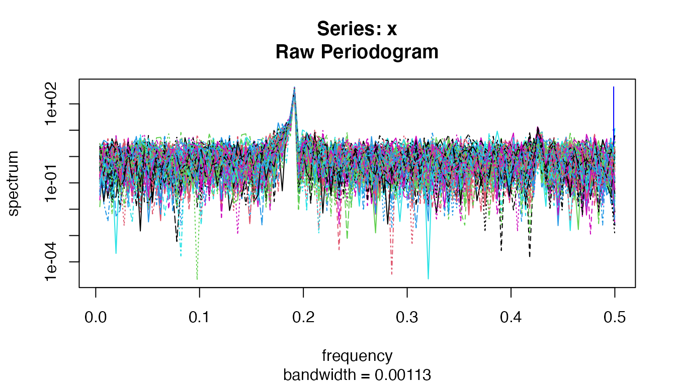
The spectrum estimation of C1.
spectrum(d2)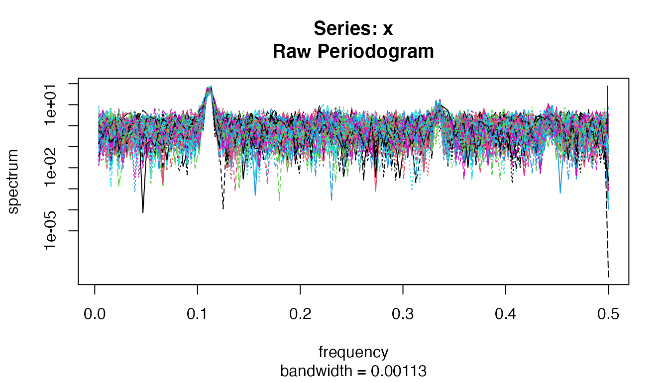
The spectrum estimation of C2.
spectrum(d3)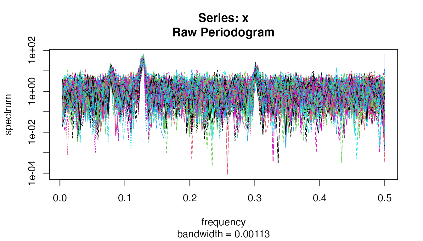
The spectrum estimation of C3.
It is expected that \(C_3\)’s bicoherence shows no outstanding pair of frequencies as \(C_3\) does not have any big component of frequency \(\frac{1.2}{2 \pi}\) nor \(\frac{0.7}{2 \pi}\), but of frequency \(\frac{0.8}{2 \pi}\) and \(\frac{1.2+0.7}{2 \pi}\) only:
bc3 <- bicoherence(d3)
heatmap_bicoherence(bc3)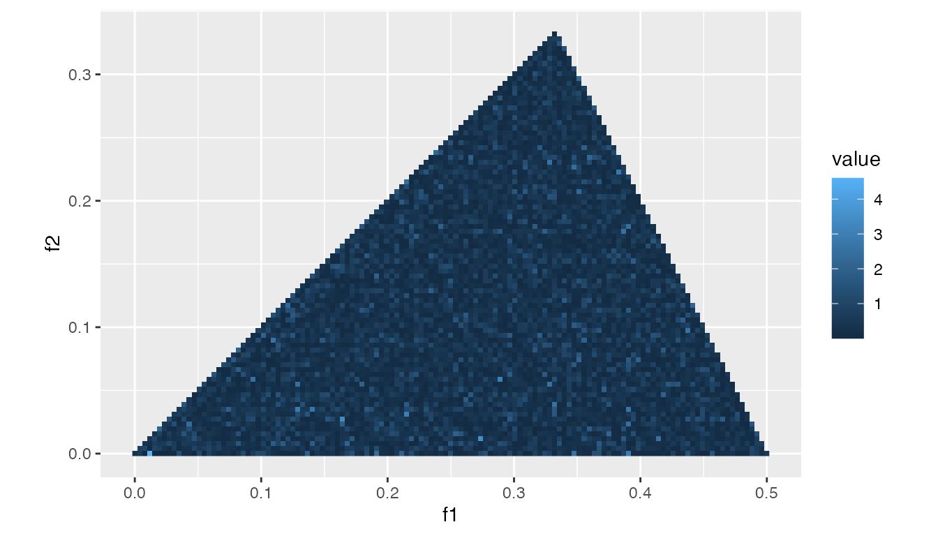
d3’s estimated bicoherence.
Now we calculate the estimated cross-bicoherence between \(C_1\), \(C_2\), and \(C_3\) by cross_bicoherence,
and plot the heat map of the results:
cb123 <- cross_bicoherence(d1, d2, d3)

heatmap_cross_bicoherence <- function(cb) {
    ggplot(cb) +
        geom_raster(aes(f1, f2, fill = value)) +
        coord_fixed() +
        scale_alpha(guide = "none")
}

heatmap_cross_bicoherence(cb123)
#> Warning: Raster pixels are placed at uneven horizontal intervals and will be shifted
#> ℹ Consider using `geom_tile()` instead.
The estimated cross-bicoherence between C1, C2, and C3.
Notice the high values around bifrequencies \((f_1, f_2) = (\frac{1.2}{2 \pi}, \frac{0.7}{2 \pi}) \approx (0.191, 0.111)\) and \((f_1, f_2) = (\frac{1.2}{2 \pi}, -\frac{0.7}{2 \pi}) \approx (0.191, -0.111)\). It means that the QPC in the model is correctly identified.
How about changing the order of cross-bicoherence’s arguments? Let’s estimate the one between \(C_3\), \(C_1\), and \(C_2\):
cb312 <- cross_bicoherence(d3, d1, d2)
heatmap_cross_bicoherence(cb312)
#> Warning: Raster pixels are placed at uneven horizontal intervals and will be shifted
#> ℹ Consider using `geom_tile()` instead.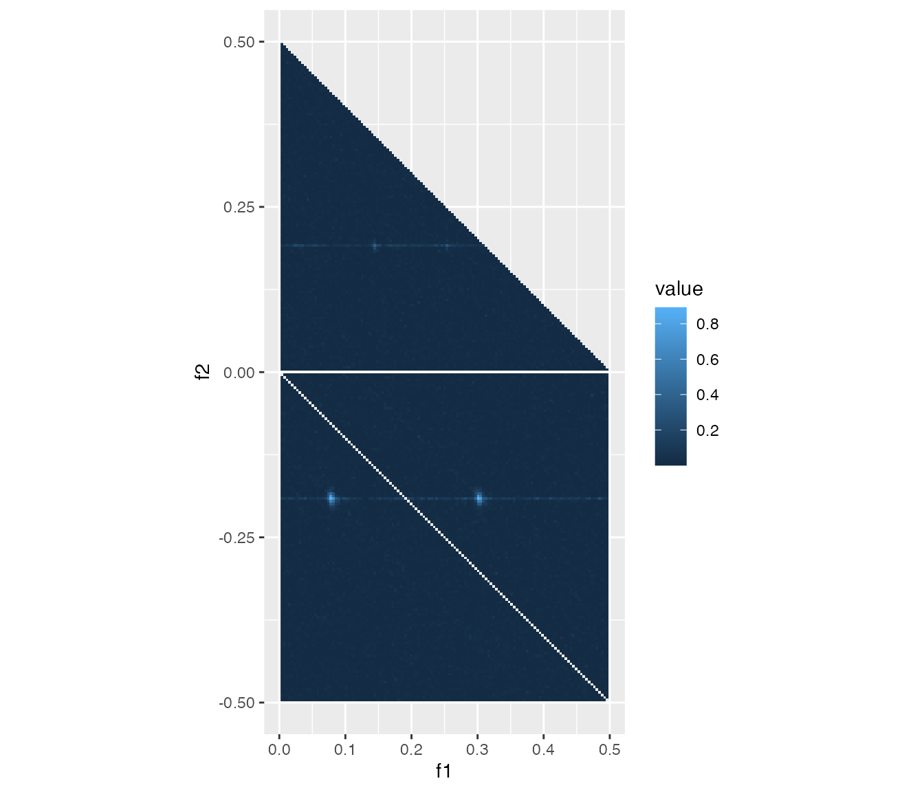
The estimated cross-bicoherencde between C3, C1, and C2.
Now the pairs of frequencies \((f_1, f_2) = (\frac{1.2-0.7}{2 \pi}, -\frac{1.2}{2 \pi}) \approx (0.080, -0.191)\) and \((f_1, f_2) = (\frac{1.2+0.7}{2 \pi}, -\frac{1.2}{2 \pi}) \approx (0.302, -0.191)\) are in highlights.
When and why existing QPC is not apparent from the estimated cross-bicoherence
Using the three-channel model in the previous section, let’s see some examples of QPC which does not exhibit a higher value of the coupling bifrequency in problem.
The most straightforward reason of invisible QPC is the weakness of
the coupling strength. It is reproducible by taking a small
Qcoef in our model.
Qcoef <- 0.01

y2 <- sample_tc()
cb2 <- cross_bicoherence(c1_data_frame(y2), c2_data_frame(y2), c3_data_frame(y2))
heatmap_cross_bicoherence(cb2)
#> Warning: Raster pixels are placed at uneven horizontal intervals and will be shifted
#> ℹ Consider using `geom_tile()` instead.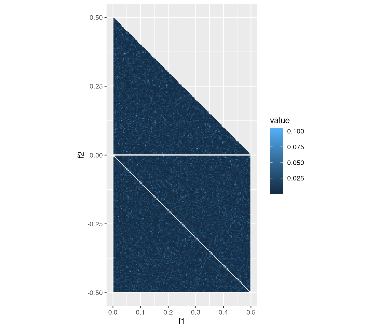
The case of weak coupling.
Another reason of undetectable QPC is that the coupling bifrequency
is in the outside of the region sufficiently sampled. The following
example demonstrates that the f1 of the bifrequency almost
equals to the Nyquist frequency. If Fcoef1 exceeds \(\pi\), it will be no longer
identifiable.
Fcoef1 <- pi - 0.1
Fcoef2 <- 2.3
Fcoef3 <- 1.5
Qcoef <- 0.3

y3 <- sample_tc()
cb3 <- cross_bicoherence(c1_data_frame(y3), c2_data_frame(y3), c3_data_frame(y3))
heatmap_cross_bicoherence(cb3)
#> Warning: Raster pixels are placed at uneven horizontal intervals and will be shifted
#> ℹ Consider using `geom_tile()` instead.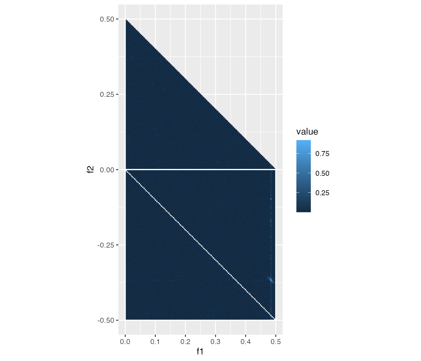
The case of nearly-Nyquist frequency of f1.
Last but not least, undersampling also ends up with missing QPC. If
the number of samples N2 is too small, we cannot
distinguish the coupling bifrequency from the others.
Fcoef1 <- 1.2
Fcoef2 <- 0.7
Fcoef3 <- 0.8
Qcoef <- 0.3
N2 <- 10

y4 <- sample_tc()
cb4 <- cross_bicoherence(c1_data_frame(y4), c2_data_frame(y4), c3_data_frame(y4))
heatmap_cross_bicoherence(cb4)
#> Warning: Raster pixels are placed at uneven horizontal intervals and will be shifted
#> ℹ Consider using `geom_tile()` instead.
The case of insufficient sample.
Conclusion
Using numerical simulation of time series of stationary stochastic
processes, we have demonstrated that rhosa’s bicoherence
and cross_bicoherence can suggest the bifrequencies of
potential QPC. Although some assumptions on the time series,
e.g. stationarity, must be satisfied for accurate estimation, there is
no additional cost except for the computing time if the first-order
spectral analysis has been adopted already. The API lowers the barrier
preventing from applying the bispectral analysis to time series for an
exploratory purpose. Considering appropriate generative models helps
interpretation of the result obtained from the analysis.
References
[1] Petropulu, A.P., 1994. Higher-Order Spectra in Biomedical Signal Processing. IFAC Proceedings Volumes, IFAC Symposium on Modelling and Control in Biomedical Systems, Galveston, TX, USA, 27-30 March 1994 27, 47–52. https://doi.org/10.1016/S1474-6670%2817%2946158-1