This is a simple example, based on the outline at Figure 1 of (Villa and Tetko 2010), which demonstrates how to use rhosa’s functions to find an obscure relationship between two frequencies in some time series imitated by a generative model.
With four cosinusoidal waves having arbitrarily different phases
(omega_a, omega_b, omega_c, and
omega_d), but sharing a couple of frequencies
(f_1 and f_2), we define function
D(t) to simulate a pair of time series: v and
w. We make them noisy by adding an independent random
variate that follows the standard normal distribution.
set.seed(1)
f_1 <- 0.35
f_2 <- 0.2
D <- function(t) {
    omega_a <- runif(1, min = 0, max = 2 * pi)
    omega_b <- runif(1, min = 0, max = 2 * pi)
    omega_c <- runif(1, min = 0, max = 2 * pi)
    omega_d <- runif(1, min = 0, max = 2 * pi)
    wave_a <- function(t) cos(2 * pi * f_1 * t + omega_a)
    wave_b <- function(t) cos(2 * pi * f_2 * t + omega_b)
    wave_c <- function(t) cos(2 * pi * f_1 * t + omega_c)
    wave_d <- function(t) cos(2 * pi * f_2 * t + omega_d)
    curve_v <- function(t) wave_a(t) + wave_b(t) + wave_a(t) * wave_b(t)
    curve_w <- function(t) wave_c(t) + wave_d(t) + wave_c(t) * wave_b(t)
    data.frame(v = curve_v(t) + rnorm(length(t)),
               w = curve_w(t) + rnorm(length(t)))
}
Both v and w are oscillatory in
principle:
data <- D(seq_len(2048))
with(data, {
    plot(seq_len(100), head(v, 100), type = "l", col = "green", ylim = c(-3, 3), xlab = "t", ylab = "value")
    lines(seq_len(100), head(w, 100), col = "orange")
})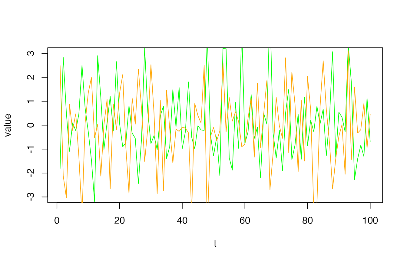
v and w.
It is noteworthy that the power spectrum densities of v
and w are basically identical as shown in their spectral
density estimation:
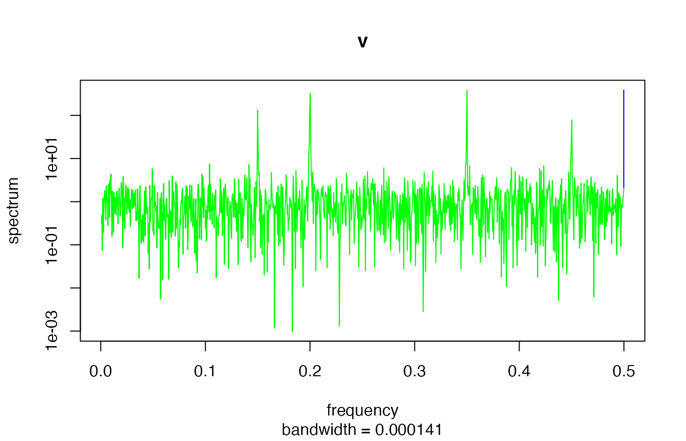
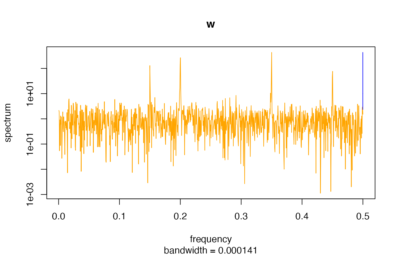
Spectral density estimation via periodograms.
On the other hand, their bispectra are different. More specifically,
we are going to see that their bicoherence at some pairs of frequencies
are different. rhosa’s bicoherence function allows us to
estimate the magnitude-squared bicoherence from samples.
x <- replicate(100, D(seq_len(128)), simplify = FALSE)
m_v <- do.call(cbind, Map(function(d) {d$v}, x))
m_w <- do.call(cbind, Map(function(d) {d$w}, x))

library(rhosa)

bc_v <- bicoherence(m_v, window_function = 'hamming')
bc_w <- bicoherence(m_w, window_function = 'hamming')
In the above code, we take 100 samples of the same length for a
smoother result. The bicoherence function accepts a matrix
whose column represents a sample sequence, and returns a data frame.
Note that an optional argument to bicoherence is given for
requesting tapering with Hamming window
function.
library(ggplot2)

plot_bicoherence <- function(bc) {
    ggplot(bc, aes(f1, f2)) +
        geom_raster(aes(fill = value)) +
        scale_fill_gradient(limits = c(0, 10)) +
        coord_fixed()
}
The axis f1 and f2 represent normalized
frequencies in unit cycles/sample of range [0, 1).
Frequency pairs of bright points in the following plot of
bc_v indicate the existence of some quadratic phase
coupling, as expected:
plot_bicoherence(bc_v)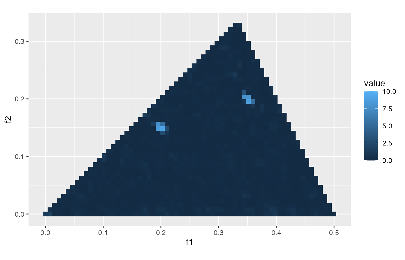
v’s estimated magnitude-squared bicoherence.
In contrast, bc_w has no peaks at frequency pair
(f_1, f_2) = (0.35, 0.2), etc.:
plot_bicoherence(bc_w)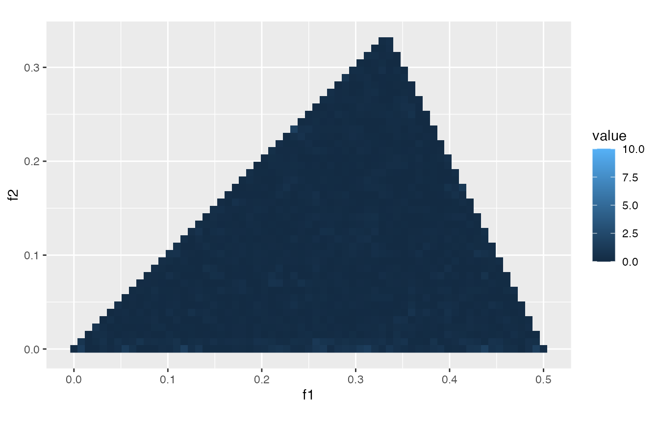
w’s estimated magnitude-squared bicoherence.